45 google sheets axis labels
› charts › switch-axisHow to Switch (Flip) X & Y Axis in Excel & Google Sheets Switching X and Y Axis. Right Click on Graph > Select Data Range . 2. Click on Values under X-Axis and change. In this case, we’re switching the X-Axis “Clicks” to “Sales”. Do the same for the Y Axis where it says “Series” Change Axis Titles. Similar to Excel, double-click the axis title to change the titles of the updated axes. Add & edit a chart or graph - Computer - Google Docs Editors … On your computer, open a spreadsheet in Google Sheets. Double-click the chart you want to change. At the right, click Customize. Click Chart & axis title. Next to "Type," choose which title you want to change. Under "Title text," enter a title. Make changes to the title and font. Tip: To edit existing titles on the chart, double-click them.
Google sheets chart tutorial: how to create charts in google ... - Ablebits Aug 15, 2017 · How to Edit Google Sheets Graph. So, you built a graph, made necessary corrections and for a certain period it satisfied you. But now you want to transform your chart: adjust the title, redefine type, change color, font, location of data labels, etc. Google Sheets offers handy tools for this. It is very easy to edit any element of the chart.
Google sheets axis labels
› dynamic-charts-google-sheetsStep-by-step guide on how to create dynamic charts in Google ... Feb 24, 2016 · Select a column chart and ensure that Column E and row 1 are marked as headers and labels: Click insert. Test your chart. It should now be dynamic so that it changes whenever you select a new name from the Google Sheets drop-down menu: Great job! You’ve now created your first of many dynamic charts in Google Sheets! › charts › horizontal-valuesHow to Change Horizontal Axis Values – Excel & Google Sheets We’ll start with the date on the X Axis and show how to change those values. Right click on the graph; Select Data Range . 3. Click on the box under X-Axis. 4. Click on the Box to Select a data range . 5. Highlight the new range that you would like for the X Axis Series. Click OK. Final Graph with Updated X Value Series in Google Sheets support.google.com › docs › answerAdd data labels, notes, or error bars to a chart - Google You can add data labels to a bar, column, scatter, area, line, waterfall, histograms, or pie chart. Learn more about chart types. On your computer, open a spreadsheet in Google Sheets. Double-click the chart you want to change. At the right, click Customize Series. Check the box next to “Data labels.”
Google sheets axis labels. How to Make a Box Plot in Google Sheets - Statology Oct 01, 2020 · Within the Customize subsection of the Chart Editor window on the right side of the screen you can also modify the plot to include titles, adjust gridlines, and modify the axis labels. Additional Resources. The following tutorials explain how to create other common charts in Google Sheets: How to Create a Pie Chart in Google Sheets Dates and Times | Charts | Google Developers Jul 07, 2020 · Overview. The date and datetime DataTable column data types utilize the built-in JavaScript Date class.. Important: In JavaScript Date objects, months are indexed starting at zero and go up through eleven, with January being month 0 and December being month 11. Dates and Times Using the Date Constructor Dates Using the Date Constructor. To create a new Date … › charts › move-horizontalMove Horizontal Axis to Bottom – Excel & Google Sheets Moving X Axis to the Bottom of the Graph. Click on the X Axis; Select Format Axis . 3. Under Format Axis, Select Labels. 4. In the box next to Label Position, switch it to Low. Final Graph in Excel. Now your X Axis Labels are showing at the bottom of the graph instead of in the middle, making it easier to see the labels. support.google.com › docs › answerAdd & edit a chart or graph - Computer - Google Docs Editors Help On your computer, open a spreadsheet in Google Sheets. Double-click the chart you want to change. At the right, click Customize. Click Chart & axis title. Next to "Type," choose which title you want to change. Under "Title text," enter a title. Make changes to the title and font. Tip: To edit existing titles on the chart, double-click them.
sheetsformarketers.com › how-to-add-axis-labels-inHow To Add Axis Labels In Google Sheets - Sheets for Marketers One common change is to add or edit Axis labels. Read on to learn how to add axis labels in Google Sheets. Insert a Chart or Graph in Google Sheets. If you don’t already have a chart in your spreadsheet, you’ll have to insert one in order to add axis labels to it. Here’s how: Step 1. Select the range you want to chart, including headers ... How to Switch (Flip) X & Y Axis in Excel & Google Sheets Switching X and Y Axis. Right Click on Graph > Select Data Range . 2. Click on Values under X-Axis and change. In this case, we’re switching the X-Axis “Clicks” to “Sales”. Do the same for the Y Axis where it says “Series” Change Axis Titles. Similar to Excel, double-click the axis title to change the titles of the updated axes. How to Create a Pie Chart in Google Sheets - Lido.app Click here to learn how to add the title, axis labels, or change the colors. How to create a 3D pie chart. Another type of pie chart that you can create in Google Sheets is the 3D pie chart. Just like pie chart and doughnut chart, the choice of using a 3D pie chart depends on the aesthetics. support.google.com › docs › answerAdd data labels, notes, or error bars to a chart - Google You can add data labels to a bar, column, scatter, area, line, waterfall, histograms, or pie chart. Learn more about chart types. On your computer, open a spreadsheet in Google Sheets. Double-click the chart you want to change. At the right, click Customize Series. Check the box next to “Data labels.”
› charts › horizontal-valuesHow to Change Horizontal Axis Values – Excel & Google Sheets We’ll start with the date on the X Axis and show how to change those values. Right click on the graph; Select Data Range . 3. Click on the box under X-Axis. 4. Click on the Box to Select a data range . 5. Highlight the new range that you would like for the X Axis Series. Click OK. Final Graph with Updated X Value Series in Google Sheets › dynamic-charts-google-sheetsStep-by-step guide on how to create dynamic charts in Google ... Feb 24, 2016 · Select a column chart and ensure that Column E and row 1 are marked as headers and labels: Click insert. Test your chart. It should now be dynamic so that it changes whenever you select a new name from the Google Sheets drop-down menu: Great job! You’ve now created your first of many dynamic charts in Google Sheets!
32 How To Label Vertical Axis In Excel - Labels Database 2020

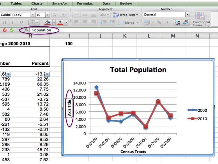
Formatting Axis Labels
30 Chart Js Axis Label - Labels Design Ideas 2020
32 How To Label A Line Graph - Labels For Your Ideas
Post a Comment for "45 google sheets axis labels"