38 how to add data labels on excel

Add a label or text box to a worksheet - support.microsoft.com Add a label (Form control) Click Developer, click Insert, and then click Label . Click the worksheet location where you want the upper-left corner of the label to appear. To specify the control properties, right-click the control, and then click Format Control. Add a label (ActiveX control) Add a text box (ActiveX control) Show the Developer tab how to add data labels into Excel graphs - storytelling with data You can download the corresponding Excel file to follow along with these steps: Right-click on a point and choose Add Data Label. You can choose any point to add a label—I'm strategically choosing the endpoint because that's where a label would best align with my design. Excel defaults to labeling the numeric value, as shown below.

Adding Data Labels to Your Chart (Microsoft Excel) For instance, if you are formatting a pie chart, the data can be more difficult to understand if you don't include data labels. To add data labels, follow these steps: Activate the chart by clicking on it, if necessary. Choose Chart Options from the Chart menu. Excel displays the Chart Options dialog box. Make sure the Data Labels tab is selected.

How to add data labels on excel

Add / Move Data Labels in Charts - Excel & Google Sheets Adding Data Labels Click on the graph Select + Sign in the top right of the graph Check Data Labels Change Position of Data Labels Click on the arrow next to Data Labels to change the position of where the labels are in relation to the bar chart Final Graph with Data Labels How To Add Data Labels In Excel * English4room The column chart will appear. For example, this is how we can add labels to one of the data series in our excel chart: Source: . Click the + symbol and add data labels by clicking it as shown below step 3: Click add chart element and select data labels, and then select a location for the data label option. Source: Add data labels to your Excel bubble charts | TechRepublic Right-click the data series and select Add Data Labels. Right-click one of the labels and select Format Data Labels. Select Y Value and Center. Move any labels that overlap. Select the data labels...

How to add data labels on excel. How To Add Data Labels In Excel } Esse 2022 Then Click The Chart Elements, And Check Data Labels, Then You Can Click The Arrow To Choose An Option About The Data Labels In The Sub Menu. Data labels are used to display source data in a chart directly. Click the chart elements button, and select the data labels option. 3d maps excel 2016 add data labels. Format Data Labels in Excel- Instructions - TeachUcomp, Inc. To do this, click the "Format" tab within the "Chart Tools" contextual tab in the Ribbon. Then select the data labels to format from the "Chart Elements" drop-down in the "Current Selection" button group. Then click the "Format Selection" button that appears below the drop-down menu in the same area. Adding Data Labels to Your Chart (Microsoft Excel) To add data labels in Excel 2013 or Excel 2016, follow these steps: Activate the chart by clicking on it, if necessary. Make sure the Design tab of the ribbon is displayed. (This will appear when the chart is selected.) Click the Add Chart Element drop-down list. Select the Data Labels tool. How to Add Total Data Labels to the Excel Stacked Bar Chart Step 4: Right click your new line chart and select "Add Data Labels" Step 5: Right click your new data labels and format them so that their label position is "Above"; also make the labels bold and increase the font size. Step 6: Right click the line, select "Format Data Series"; in the Line Color menu, select "No line" Step 7 ...

Labels - How to add labels | Excel E-Maps Tutorial You can add a label to a point by selecting a column in the LabelColumn menu. Here you can see an example of the placed labels. If you would like different colors on different points you should create a thematic layer. You can do this by following the tutorial about Thematic Points and to chooce Individual Colors. You can find the tutorial here. Custom Chart Data Labels In Excel With Formulas Follow the steps below to create the custom data labels. Select the chart label you want to change. In the formula-bar hit = (equals), select the cell reference containing your chart label's data. In this case, the first label is in cell E2. Finally, repeat for all your chart laebls. Excel tutorial: How to use data labels When you check the box, you'll see data labels appear in the chart. If you have more than one data series, you can select a series first, then turn on data labels for that series only. You can even select a single bar, and show just one data label. In a bar or column chart, data labels will first appear outside the bar end. How to Add Data Labels in Excel - Excelchat | Excelchat How to Add Data Labels In Excel 2013 And Later Versions In Excel 2013 and the later versions we need to do the followings; Click anywhere in the chart area to display the Chart Elements button Figure 5. Chart Elements Button Click the Chart Elements button > Select the Data Labels, then click the Arrow to choose the data labels position. Figure 6.

Add data labels and callouts to charts in Excel 365 - EasyTweaks.com The steps that I will share in this guide apply to Excel 2021 / 2019 / 2016. Step #1: After generating the chart in Excel, right-click anywhere within the chart and select Add labels . Note that you can also select the very handy option of Adding data Callouts. How to Make a Pie Chart in Excel & Add Rich Data Labels to The Chart! 7) With the data point still selected, go to Chart Tools>Format>Shape Styles and click on the drop-down arrow next to Shape Effects and select Shadow and choose Inner Shadow>Inside Diagonal Top Left. 8) With the one data point still selected, right-click this data point, and select Add Data Label>Add Data Callout as shown below. How to create Custom Data Labels in Excel Charts Create the chart as usual. Add default data labels. Click on each unwanted label (using slow double click) and delete it. Select each item where you want the custom label one at a time. Press F2 to move focus to the Formula editing box. Type the equal to sign. Now click on the cell which contains the appropriate label. Add or remove data labels in a chart - Microsoft Support To label one data point, after clicking the series, click that data point. In the upper right corner, next to the chart, click Add Chart Element > Data Labels. To change the location, click the arrow, and choose an option. If you want to show your data label inside a text bubble shape, click Data Callout.

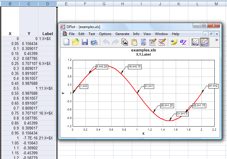
DPlot Windows software for Excel users to create presentation quality graphs

How to Customize Your Excel Pivot Chart Data Labels The Data Labels command on the Design tab's Add Chart Element menu in Excel allows you to label data markers with values from your pivot table. When you click the command button, Excel displays a menu with commands corresponding to locations for the data labels: None, Center, Left, Right, Above, and Below.

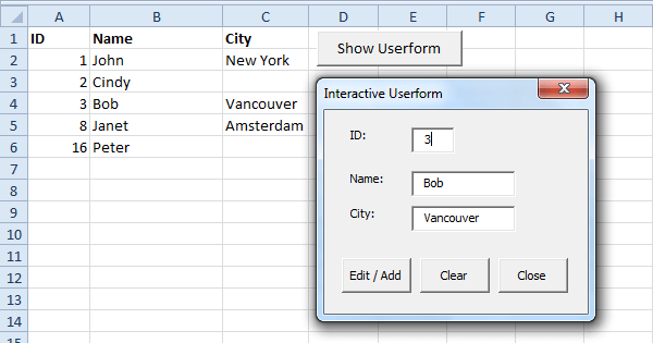
Excel VBA Interactive Userform - Easy Excel Macros

How to Print Labels From Excel - Lifewire Choose Start Mail Merge > Labels . Choose the brand in the Label Vendors box and then choose the product number, which is listed on the label package. You can also select New Label if you want to enter custom label dimensions. Click OK when you are ready to proceed. Connect the Worksheet to the Labels

Multiple Series in One Excel Chart - Peltier Tech Blog

How to add data labels in excel to graph or chart (Step-by-Step) 1. Select a data series or a graph. After picking the series, click the data point you want to label. 2. Click Add Chart Element Chart Elements button > Data Labels in the upper right corner, close to the chart. 3. Click the arrow and select an option to modify the location. 4.

Pattern fill

Add a DATA LABEL to ONE POINT on a chart in Excel Click on the chart line to add the data point to. All the data points will be highlighted. Click again on the single point that you want to add a data label to. Right-click and select ' Add data label ' This is the key step! Right-click again on the data point itself (not the label) and select ' Format data label '.

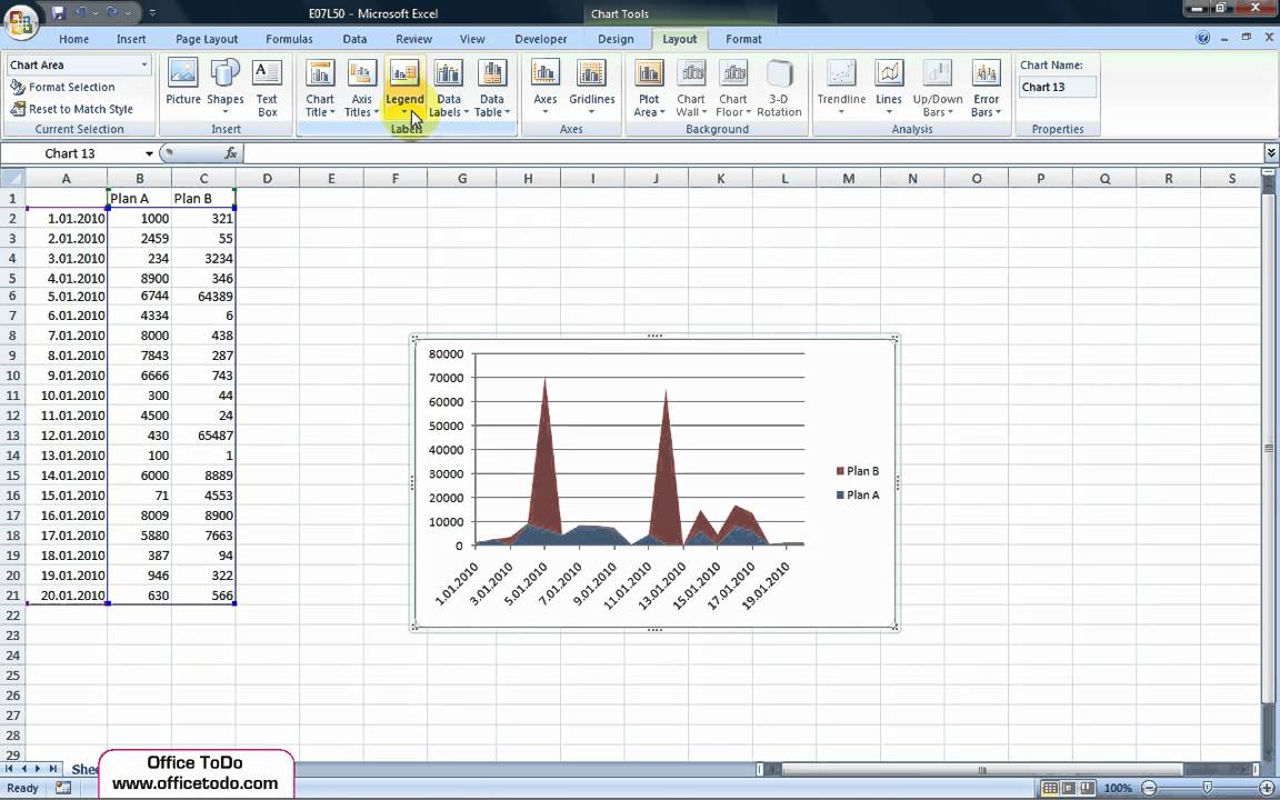
Excel | How to add, remove or reposition chart legend? - YouTube

How do I add custom labels on a dynamic graph in Excel However, I would also like the data labels to be in custom format, i.e displaying both number of units sold as well as the % of total units sold that month like this [200 (28%)] The only method I know to apply custom data labels is linking individual data labels to the excel cells. But this won't work with dynamic chart as not all rows of the ...

Mail Merge for Mac - Labels - YouTube

How to add data labels from different column in an Excel chart? Right click the data series in the chart, and select Add Data Labels > Add Data Labels from the context menu to add data labels. 2. Click any data label to select all data labels, and then click the specified data label to select it only in the chart. 3.

Share :